Risk pooling
From Supply Chain Management Encyclopedia
Russian: Объединение риска
Risk pooling involves the process of aggregating objects into a larger group whereby the risk of the group is less than the sum of risk of the individual objects. This may be mathematically expressed as:

Where:
- Oi = object i.
One of the major applications of risk pooling is in the insurance industry. However, it has also been applied in various other fields including economics and supply chain management. In economics, vertcial integration (see outsourcing) is less likely when the firm forms "a small part of total demand for the input since they would lose the risk pooling economics of large markets as they integrate. Incentives for integration may increase if the demand by other firms for inputs is highly variable, thereby driving up the price.”[1] In supply chain management, the two major applications of risk pooling center on form postponement and geographic postponement. In form postponement, the objects being aggregated are products (i.e., risk pooling across products) and its opposite is referred to as form speculation. In form postponement, action on the final form of a product uis delayed until after an order is received (see order penetration point). In geographic postponement, the objects being aggregated are geographic regions (i.e., risk pooling across space), with its corresponding opposite labeled geographic speculation. Under geographic postponement, a smaller number of warehouses are utilized. The firm thus postpones the decision of where inventory should be lpaced until after an order is received.
If the risk of the objects are independent of one another, then a high risk from one object will offset the low risk from another object. If this occurs, then risk from pooling < unpooled risk. The greater the correlation of the risk of between various objects, the smaller the difference between the risk from pooling and the unpooled risk[2]. The fundamental benefit from risk pooling in supply chain management is that lower risk loosely equates with lower variance and lower variance in a supply chain system generally equates with less safety stock. Through lower safety stock, risk pooling may lower the inventory carrying cost without sacrificing service levels. The final analysis involves a trade-off between the benefits of risk pooling (i.e., lower safety stock) and the cost of implementing the risk pooling strategy.
Example: Risk Pooling Across Products
The well known Dell example of delayed assembly until after orders arrive well illustrates the concept of assemble-to-order. Component parts are ready for assembly, however, the final configuration of the product is delayed (or postponed) until after orders have arrived. HP illustrates the strategy of form speculation: products are made-to-stock based on forecasting (see order penetration point). Supposed a company manufacturers two products, SKU 4501 and 4502. The production lead time for each product is 21 days and we shall assume for expository purposes that the lead times are constant. As seen in Table 1, respective average weekly demand for the SKUs are 1200 and 2200 and respective standard deviations in weekly demand are 170 and 230. Using the inventory model with uncertainty in demand and lead time provides respective average safety stock levels of 1,597 amd 2,161, for a total average safety stock level of 3,758.
| Table 1: Unpooled Risk (Form Speculation); In-stock probability = 98% (z=2.05) | ||
|---|---|---|
| Product | SKU 4501 | SKU 4502 |
| Production lead time in days = L | 21 | 21 days |
| Average weekly demand | 1200 | 2200 |
| Standard deviation in weekly demand = SD | 170 | 230 |
| Safety stock = z × SD √ L | 2.05 × 170 √21 = 1,597 | 2.05 × 230 √21 = 2,161 |
| Total amount of safety stock = 1,597 + 2,161 = 3,758 | ||
Now suppose that the firm examines an alternative policy based on the idea that the majority of product is common to both SKUs. The production lead time for the common "base" product is 20 days and, as seen in Table 2, just one day is required for the final configuration of both SKUs. The standard deviation of demand for the "base" product equals the square root of the sum of the standard deviations of demand squared. This assumes that Var(X+Y) = Var(X) + Var(Y). This is where the risk pooling concept comes into effect. From a statistical persepctive, the Var(X+Y) = Var(X) + Var(Y) + 2Covariance(X,Y). In other words, we are assuming that the demand for the two SKUs is independent and that the Cov(SKU 5401, SKU 4502)=0. The analysis shown in Table 2 therefore represents the "best case" scenario in terms of reduction in safety stock resulting from risk pooling or form postponement given the values of the remaining parameters in this model. The remainder of the analysis is similar to that shown in Table 1. Safety stock is evaluated for the "base" product as well as for the two finished SKUs. The sum equals 3,442, which therefore represents a "best case" reduction of 8.40% of inventory.
| Table 2: Pooled Risk (Form Postponement); In-stock probability = 98% (z=2.05) | |||
|---|---|---|---|
| Product | Base Product | SKU 4501 | SKU 4502 |
| Production lead time in days = L | 20 | 1 | 1 |
| Average weekly demand | 3400 | 1200 | 2200 |
| Standard deviation in weekly demand = SD | √ (170² + 230²) = 286 | 170 | 230 |
| Safety stock = z × SD √ L | 2.05 × 286 √20 = 2,622 | 2.05 × 170 √1 = 349 | 2.05 × 230 √1 = 472 |
| Total amount of safety stock = 2,622 + 349 + 472 = 3,442 | |||
| Percentage reduction in safety stock = (3,758 - 3,422) / 3,758 = 8.40% | |||
One cannot conclude from the this analysis that form postponement always leads to a reduction in safety stock. With the assumption that demand across products is independent, the general formula utilized in Tables 1 and 2 is expressed as:
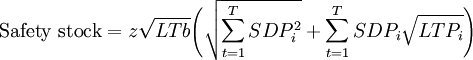
Where:
- LTb = Production lead time for base product
- LTPi = Production lead time for product i (in this case LTb + LTPi must be contrained to 21)
- SDPi = Standard deviation in demand for product i
We may then evaluate the change in safety stock for alternative base product production lead times. As seen in Table 3, only when the base product production lead time equals 19 and 20 days does the level of safety stock decline (by 1% and 8% resepctively). The relationship between base product production lead time and change in safety stock is shown in Chart 1. For all other base product production lead times, safety stock inventory increases relative to the case of no risk pooling (or complete form speculation as shown in Table 1). In these instances, the firm should consider a make-to-stock orientation.
| Table 3: Percentage change (+/-) in Safety Stock at Various Base Product Production Lead Times; In-stock probability = 98% (z=2.05) | |||||||||||||||||||||
|---|---|---|---|---|---|---|---|---|---|---|---|---|---|---|---|---|---|---|---|---|---|
| Base product production lead time (days) | 1 | 2 | 3 | 4 | 5 | 6 | 7 | 8 | 9 | 10 | 11 | 12 | 13 | 14 | 15 | 16 | 17 | 18 | 19 | 20 | |
| Percentage change (+/-) in safety stock | 13% | 17% | 20% | 21% | 22% | 23% | 23% | 23% | 22% | 22% | 21% | 20% | 18% | 16% | 14% | 11% | 8% | 4% | -1% | -8% | |
Example: Risk Pooling Across Space - The Square Root Rule
Risk pooling across space suggests that the objects being aggregated are geographic regions. This is equivalent to geographic postponement since the firm delays descions on where products are needed until after orders have arrived. The primary operationalization of risk pooling across space is through the use of fewer warehouses. Similar to the case of risk pooling across products, the extent of risk reduction will depend on the covariation of demand (positive, negative, null) among the regions. The general experience of the business community is that risk pooling across space associates with lower variance in demand. This ultimately leads to lower safety stock inventory. A heuristic that captures the reduction in demand from risk pooling across space is known as the square root rule[3].
Square Root Rule

Where:
- If = Total inventory at future facilities
- nc = number of current facilities
- nf = number of future facilities
If a business operates five warehouses and the value of inventory at each warehouse equals €100,000, then the total value of inventory equals 5 × €100,000 = €500,000. How much inventory would be needed if one warehouse were operated?
- Given: Ic = €500,000; nc = 5; nf = 1
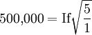
- Therefore, If = €223,607
- This represents a 55% reduction in inventory
The reduction in invetory from risk pooling across space was obtained through a decline in safety stock. The economic argument for a reduction in the number of warehouses requires a total cost analysis as the use of fewer warehouses may lead to a shift in the underlying transportation cost structrure. Furthermore, the square root rule is a simplified model that assumes: (1) transshipments between facilities is not common; (2) lead times variance is neglible; (3) the service levels across facilities is constant; and (4) the distribution of demand at the facilities is normal.
References
- ↑ Carlton, D.W. (1979), “Vertical Integration in Competitive Markets under Uncertainty,” Journal of Industrial Economics, 27 (3), p.204.
- ↑ Simchi-Levi, D., P. Kaminsky and E. Simchi-Levi (2000), Designing and Managing the Supply Chain, Irwin Mc-Graw Hill, Boston, p.56-60.
- ↑ Zinn, W; M. Levy, and D.J. Bowersox (1989), "Measuring the Effect of Inventory Centralization/Decentralization on Aggregate Safety Stock: The "Square Root Law" Revisited", Journal of Business Logistics, 10 (1), 1-14.