Network models
From Supply Chain Management Encyclopedia
Russian: Сетевые модели
The Main Definitions
Let  is a finite set called a set of nodes. The rule
  , which associates each element
  with an element
  , is called single-valued transformation
  in . A multi-valued transformation
  of the set in is a rule that for each element defines a subset
  (in this case it is allowed
  ) .
A couple
) .
A couple  is called a graph if is a finite set, a is a transformation of in . As an example, consider a supply chain in which suppliers, manufacturers and consumers of all levels are the nodes of the graph, and transformation describes all possible routes for the movement of materials (goods).
Further elements of will be represented by points on the plane, and a pair of points  and
and  , for which
  , will be joined by continuous line with an arrow pointing from to . Each element of is called a vertex or node of the graph, and a pair of elements
  , where is the arc of the graph. The set of arcs in the graph is denoted by
  .
.
The set of arcs in the graph defines the mapping and vice versa, mapping defines the many . Therefore, the graph can be written in the form of , and as  .
.
An edge of the graph is the set of two elements , , for which the following conditions takes place:  , or
, or  . An edge has no an orientation . Edges are denoted by the letters
  ,
,  , the set of edges -
  .
.
A chain is a sequence of edges  , in which each edge
  has the boundary vertex for
  , the other vertex is the boundary for
  .
.
A cycle is the chain starting at some vertex and ending at the same vertex. A graph is called connected graph if any two vertices can be connected by a chain.
Network is a graph whose edge set is given by a numerical function.
Each network is associated a particular stream (e.g. gas flow in pipelines, the flow of information in computer networks). Assume that the flow in the network is limited by bandwidth of its edges, which can be both finite and infinite.
The Transportation Problem
In this section, a special class of linear programming problems - transportation models – is considered. The classical problem of transportation is the following: some goods are to be delivered from several points of origin (production, warehouses) to several destinations (customers, stores). In other words, there are two types of nodes:
1) sources (departure)
2) sinks (destinations)
In the transportation problem supply and demand are known, the cost of transportation on any route directly proportional to the volume of cargo. The problem is to find a transportation plan, in which the total transportation costs are minimal and all products are exported from the points of departure and demand at the all destination points is satisfied.
It should be noted that on the one hand the mathematical solution of transport models, is applicable to a variety of real-world problems, in which nothing will be transported (the problem of optimal assignment of employees, production planning for months, etc.). On the other hand, not all the problems of logistics of transportation are in the class of linear programming problems (traveling salesman problem, the problem of the shortest path).
2.1 Statements of the transportation problem
In this section three ways to specify the transportation problem are considered: analytical, network and a table.
- Analytical method
Consider the transportation problem in the classical statement. Let there are  points of production and
  points of consumption. Define a table of transportation costs, consisting of elements
  - the transportation cost per unit from
  -th producer to
  th customer:
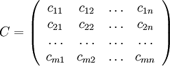 All the elements of the transport table
  are known.
Consider a transportation table, consisting of variables  - the number of transported goods from -th producer to - th customer:
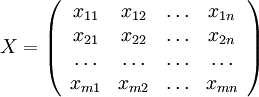
The elements of the table  are unknown. There are variables whose values are to be determined.
Production and consumption denote respectively as follows:  and
and  .
.
- Network method
The figure shows an overview of the transport problem as a network with two types of nodes, corresponding to points of origin and destinations. Arcs, connecting the nodes, correspond to routes between the origin and destination. Each arc  is defined by the costs and the amount of cargo :

- Table method
Rows of Table 2 correspond to the points of origin and the columns correspond to the points of destinations. Cells correspond to the parameters and variables . The consumption is set in the cell lines  , the volume of production - in a column
  :
:

Table 2.
2.2 Mathematical model of the transportation problem
To optimize the transportation problem we are to minimize transportation costs. Marginal costs are presented in the transportation table , the variables form a table . To create an objective function we may multiply elements of a tables and and then summarize the resulting products. The total costs are:

under constraints on departure points:
 , где
, где 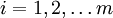
and constraints on destination points:
 , где
, где 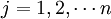
Consider also non-negativity and integer variables:
 , - integer.
2.3 Example
A company "Comfort" has two stores. Earlier this week, it received orders from three customers for 6, 7 and 11 cabinets. In the first warehouse there are 15, in the second warehouse - 9 cabinets. Replenishment is not expected. The cost of transportation of one cabinet from the first warehouse to consumers 1, 2, 3 is respectively 600, 100, 400 rubles. From the second warehouse - 1200, 200, 800 rubles respectively.
Find a transportation plan that minimizes total transportation costs.
To solve a problem consider a network:

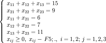
The problem is balanced, since the total inventory in the warehouses  equal to the volume of demand:
 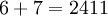 . The mathematical formulation is the following:

2.4 Balance condition of the transport model.
- Balance condition
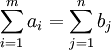
The transportation problem is balanced, if the condition of balance - the total output is equal to the total volume of consumption:
In this case, the problem has an optimal solution. Balance condition is not fulfilled in two cases: over-supply and deficit.
- Over-supply
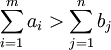
The solution in over-supply case depends on fines for incomplete removal of goods from the warehouse:
1) No fines. Therefore, the objective function (total cost) is not changed, part of the goods remains in storage. In the math formulation replace the equal sign in the restrictions on production with the inequality:
 , где
, где
, где
, - целые.
2) There are penalties for possession of the remaining goods in at least one point of departure. The size of the penalty is proportional to the number of items. In this case, the objective function includes the emerging costs. Balance the model by adding a fictitious user. We assume that the consumer has a demand 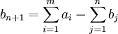 . The penalty for the remainder of departure at number denote
  . Thus, the transportation table has an additional column of traffic with the number . As a result, we have a new problem, for which the condition of balanced.
Example.
The next problem is the overproduction of four units:

The penalty for the remainder on the first warehouse is zero, for the second – is equal to 2, for the third - 1. We introduce a fictitious consumer demand with volume 4:

- Deficit

Solution of the transportation problem subject to deficit depends on the existence of penalties for unmet demand:
1) No penalties. Therefore, the objective function (total cost) is not changed, part of the goods are not delivered to customers. In the math formulation replace the equal sign in the restrictions on the volume of demand with inequality:
, where
 , where
, - integer.
2) There are penalties for unsatisfied demand, at least for one consumer. The size of the penalty is proportional to the number of units not delivered the goods. In this case, the objective function includes the emerging costs. Balance the problem by adding a fictitious manufacturer. Assume that the manufacturer has the missing amount 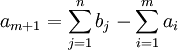 . The penalty for each unit of product, which was not delivered to the consumer , denote
  . Thus, the transportation table has the additional line . As a result, we have a new task, for which the condition of balance is hold.
Example.
In the next example deficit is equal to 7 units:

The penalty for unsatisfied demand of the first and the fourth user is zero. For the second manufacturer fee is equal to 3, for the third manufacturer - 1. Consider a fictitious manufacturer with inventory of 7 items:

2.5 Initial solution
For the correct solution of transportation problems by using an add-on for MS Excel "Solver" it is necessary to indicate an initial solution that is feasible. In this section two methods to find a feasible solution are considered. They are: method northwest element and method of a minimal element.
- Method northwest element
Algorithm:
1) For a variable in the top left table cell the maximum value allowed by the constraints on supply and demand is assigned.
2) A row (or column) with satisfied offer (or demand) is eliminated. Offer (or demand) in the corresponding row (or column) is being corrected.
3) If the table consists of only one row or only one column, its cells are filled according to the available offer and demand. Otherwise, proceed to the first stage.
Define the initial solution by the northwest elements in the transportation problem of "Comfort" company:

- Minimum element method
Algotithm:
1) In the transportation table the cell with minimal costs is determined. For a variable in this cell the maximum value allowed by the constraints on supply and demand is assigned
2) A row (or column) with satisfied offer (or demand) is eliminated. Offer (or demand) in the corresponding row (or column) is being corrected.
3) If the table consists of only one row or only one column, its cells are filled according to the available offer and demand. Otherwise, proceed to the first stage.
Define the initial solution by the minimum element method in the transportation problem of "Comfort" company:

2.6 Transportation problem solving in MS Excel

Open a sheet "feasible solution". Determine the optimal transportation plan, according to incoming orders for the company "Comfort" from the example at paragraph 2.3.
Cells containing parameters of the problem, we will be mark by blue frame. Cells containing the variables, we will mark by the red frames.
Parameters
In cells C6: E7 indicate the cost of transportation from each warehouse to each customer
In cells C12: E13 we specify the initial values of traffic volume, determined by the method of minimum element.
Cells H12: H13 indicate the existing product inventories in warehouses
In cells C16: E16 we set the value of customers' 1, 2 and 3 order volumes
Restrictions
In cell F12 calculate the total amount of goods exported from the first store using the formula:
=SUM(C12:E12).
In cell F13 indicate the total quantity of goods exported from the second warehouse.
Similarly, we define the number of goods delivered to each customer. In a cell C14 count the total number of goods delivered to the first client using the formula:
=SUM(C12:C13).
To determine the number of products received the second and third clients, copy the formula in cell D14: E14. Note that in this case we use relative addressing.
Objective function
In cell C20 we calculate the total cost of transportation problem using the formula:
=SUMPRODUCT(C6:E7;C12:E13).
Solver
Open a sheet "optimal solution" and open the add-in "Solver".
Set Target Cell. Specify the cell C20 - the total cost
Variable cell. Select the array $C$12:$E$13 as changing cells.
Restrictions. Add restrictions on the available inventory: $F$12:$F$13 = $H$12:$H$13 on demand: $C$14:$E$14 = $C$16: $E$16, and the integrality and nonnegativity of the variables: $C$12:$E$13 = integer, $C$12:$E$13.
Click the Options button and set the flag in the linear model. We return to the Solver Parameters dialog box and click Run.
The total cost of transportation is 10200 rub. This result was unexpected for the delivery of the company "Comfort".
Recall that the initial decision obtained by a minimum element method consists in exporting of goods by the cheapest route.
Of course, in the first step it was supposed to take out the maximum number of goods from the first warehouse to the second client, because shipping is only $100. But at the same time the total transportation costs were significantly different from the optimum value and accounted for 13 500 rubles.
In addition, according to the optimal plan we not carry anything from the first warehouse to the second consumer! How can we explain that the "Solver" "ignored" in the optimal solution of the lowest cost?
It is easy to see that in the solution obtained by the method of the minimal element, the goods are carried by the cheapest route (from the first warehouse of second client), and the goods are carried by the most expensive route (from the second warehouse the first client). In this case the cost of transportation of one cabinet by the last route is 1,200 rubles, and in the solution proposed we carry 6 cabinets by this route. Now consider the optimal transportation plan. Yes, by the cheapest route we are taking nothing, but we also do not use the most expensive route.
Distribution Problem
As already noted, in a network method of defining such problems, there are two types of nodes: sources and sinks. Distribution problem is the most general statement of the network problem. It differs from the transportation model by the presence nodes of three types in a network:
1) Sources
2) Sinks
3) Intermediate nodes
As in the transportation models, each source is characterized by offer, stock – by demand. Intermediate nodes have zero demand and supply. Consequently, the distribution problem includes, as a special case, a transportation model.
3.1 Mathematical formulation of the distribution problem
Introduce the following notation:
- the set of nodes;
- the number of nodes,
- the set of arcs,
- flow passing through the arc ,
- costs of unit of flow from to ,
 - lower bound of flow from to ,
 - upper bound of flow from to ,
 - capacity in the node ,
 - arc.
Consider the level of demand in the sink as a performance with a minus sign. This allows writing the condition of the balance model in the form:

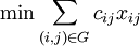
Objective function
Consider the problem of finding a flow of minimal value in a network. The objective function becomes:
Restrictions
1) Restrictions defined by bandwidth of edges
Each variable defines the flow flowing along the edge , therefore, it must satisfy the constraints on the bandwidth of the edge:

For each node it must be satisfied the basic relation for the flow
2) The basic relation for the flow
For each network node it must hold:
The effluent - Inflowing flow = Node capacity
Or in the notation:
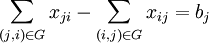 ,
, 
In addition, it should be satisfied non-negativity and integrality conditions:
- integer.
Finally, mathematical statement has the following form:

,
- integer.
3.1. The problem of minimal route
The problem of minimal route is the problem of determination the shortest path between two nodes of the transport network. Many real tasks such as routing, equipment replacement schedule, the load problem can be formalized by this model.
Example.
A "Comfort" company has received from non-resident client order for production and delivery of exclusive table. The department of logistics of the company has a map of roads with distances between towns:

A company "Comfort" is located in the city 1, the destination is the city 7. The table was made in time, the company needs to find a route of minimum length.
Solution.
Let's start by checking the balance of the model. The firm has received an order for a table. Recall that demand is treated as a negative performance; therefore, the balance condition is satisfied:
Let is a flow from the city to the city . The cost are the distances between cities, then the objective function becomes:


Restrictions on the bandwidth problem are not defined, that is, all the roads can carry any amount of cargo.
Consider the basic relations for a flow. The first node is the source from which it is possible to get into the city 2, 3 and 4. Order quantity is one unit, then the performance of the source is 1. Influent flow is absent, thus:
 (узел 1)
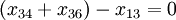
Consider the basic relation for the intermediate network nodes. It is known that their performance is equal to zero. From the city 2 is possible to get only city 4 and 5. Get into the city 2 it is possible only from the city of 1. It means that the basic relation of the node 2 has the form:
 (node 2)
For the rest nodes we get:
 (node 3)
 (node 4)
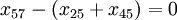 (node 5)
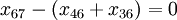 (node 6)
A node 7 can be reached from nodes 4, 5 and 6. The effluent from the node 7 is missing. Considering the negative performance of demand, we have:
 (node 7).
Take into account non-negativity and integrality of the flow:
, - integer.
3.2. The realization of the problem of minimal route in MS Excel


Open a sheet "feasible solution". We define the shortest path, according to the pattern of roads in the example of paragraph 3.1.
As before, cells containing the parameters of the problem will be marked by blue frame. Cells that contain variables, mark by the red frames.
{\bf Parameters}
In cells B8: M8 specify the distance between cities
In cells B9: M15 indicate the coefficients corresponding to the effluent and influent stream in each node. It is sufficient to specify only the values 1 and -1. The contents of the empty cells are interpreted as 0.
Cells P9: P15 indicate the performance of nodes
In cells B6: M6 specify any feasible path between the source and sink, for example, 1> 2> 5> 7. To realize this it is necessary to set the value of a variable  ,
,  ,
,  . Other variables set to zero.
Restrictions
The cell N9 indicates the total flow flowing from node 1:
=SUMPRODUCT($B$6:$M$6;B9:M9).
Here we use absolute addressing for the array of cells containing the variables of the problem: $B$6:$M$6, and relative addressing for the coefficients: B9:M9. This allows to copy the formula into the cell corresponding to the remaining nodes: N10: N15.
Objective function
In cell A19 calculate the total path length using the formula:
= SUMPRODUCT (C6:E7;C12:E13).
The path length 1> 2> 5> 7 equals 80.
Solver
On the sheet "optimal solution", open the add-in "Solver".
Set Target Cell. Specify the cell A19 - the path length
Variable cell. Select the array $B$6:$M$6 as the changing cells.
Restrictions. Add restrictions on the value flowing and inflowing streams for each of the seven nodes: $N$9:$N$15 = $P$9:$P$15, and the integrality and nonnegativity of the variables: $B$6:$M$6 = integer, $B$6:$M$6.
Click the Options button and set the flag in the linear model. Return to the Solver Parameters dialog box and click Run.
As a result of optimizing the unit values have been assigned to the following variables:  ,
,  ,
,  . The remaining variables are zero. This corresponds to path 1> 3> 6> 7. The length of this path is specified in the target cell and is equal to 68.
Network interpretation of the solution:
Note that in the problem of "Comfort" company was to bring the customer one exclusive table. Of course, the optimization problem solution (finding the shortest path) does not depend on order volume. Therefore, the general formulation of the problem of the shortest path is always assumed that the performance of the source (or sink) is equal to 1 (minus 1).