Inventory model with uncertainty in demand and lead time
From Supply Chain Management Encyclopedia
Russian: Модель запасов в условиях неопределенности
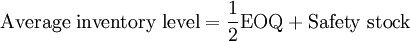
The inventory model with uncertainty in demand and lead time is designed to offer an inventory ordering policy that includes a reorder point and an order quantity when demand and lead time are not constant.[1] The assumptions of the model are that demand and lead time are normally distributed. The model accounts for an inventory service level, but does not include an out-of-stock penalty. The model consists of three elements: safety stock, the reorder point (RP) and the order-up-to level (OL). The reorder point and the order-up-to-level refer to the inventory position which is equal to the amount on of inventory on hand plus that on order. This will be demonstrated in the example provided below.


Where:
- D = average demand
- σD = standard deviation in demand
- LT = lead time
- σLT = standard deviation in lead time
- z = standard normal distribution transformation for setting the inventory service level
- EOQ = economic order quantity (provided below)
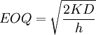
Where:
- K = fixed order cost
- D = average demand
- c = inventory carrying cost rate
- v = the relpacement value of one unit of inventory
- h = inventory carrying cost rate per unit per relevant time period
- If D is expressed annually, then h = c × v
Example
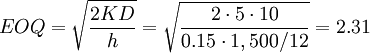
Suppose that an electric utility company consumes various types of tranformers. The utility keeps track of usage and of lead times for all the different transformer models utilized. One model has a landed cost of €1,500 per unit (v). The utility requires 10 transformers per month (D). The distribution of demand is normal with a standard deviation of 2 (σD). The lead time (LT) is 0.5 of a month (or about 15 days). It as well is normally distributed with a standard deviation of 0.10 (σLT) of a month (about 3 days). The utility wants a high service level so it selects a z value of 2.33 (or a 99% inventory service level). The actual service level in reality is higher than this as utility companies have cooperative arrangements with neighboring utilities to supply transformers if an out-of-stock situation occurs. We shall for the purpose of this example, ignore this special feature. The fixed order cost is very low as the transformer is a standard stock product that is purchased from a long term vendor. A purchasing manager for the utility receives a report each day containing the inventory position for all transformers. If the inventory position falls below the reorder point, the software flags the manager. An electronic invoice is then sent to the vendor. The fixed order cost is minimal and is estimated to be €5. The annual inventory carrying rate (c) is relatively low as obsolesence, theft, loss, and shrinkage are minimal. The carrying cost rate consists primarily of insurance, a warehousing handling fee, and the cost of capital. It is estimated to be 0.15.
What should be the order policty of the utility regarding this transformer, how much inventory will typically be on hand, and what is annual inventory hold cost per year?


Given these inputs, the reorder policy should be (9;12) - this is, when the inventory position falls below 32 units, sufficient inventory should be order to bring the inventory position back up to 36. Three issues should be raised:
- In the evaluation of the EOQ, note that the carrying cost per unit in the denominator must reflect the relevant time period. Demand and lead time were expressed in monthly terms. The carrying cost rate was expressed annually. Division of (c×v) by 12 provides the apporporiate inventory holding cost per unit per month.
- The order policy of (9;12) guarantees an inventory service level of 99%.
- The policy refers to the inventory position. Suppose that the inventory information system tracks stock on a continual basis and once a day flags are issued if orders need to be placed. Table 1 provides a hypothetical demand pattern for the public utility. On day 1, the inventory on hand is 10, demand is zero, and the inventory position (the sum of the two) equals 10. This is within the inventory policy limit set by the (9;12) rule. On day 2, demand is one unit, inventory on hand falls to 9, and the position equals 9. Again. no action is required. Day 4 demand is two units. The position, without any action would fall to 7. An order of five units is required to bring the position to its upper limit of 12. On day 6, another transformer is demanded, however, the position remains greater than or equal to 9. No action is required. One result of this is that it is possible to have multiple orders on hand, spread across a 15 day period, with orders expected to arrive every several days.
| Table 1: Illustration of Inventory Position: The Public Utility Case (9;12) | |||||
|---|---|---|---|---|---|
| Day | Demand | Inventory on Hand | Inventory on order | Action required | Inventory Position |
| 1 | 0 | 10 | 0 | None | 10 |
| 2 | 1 | 9 | 0 | None | 9 |
| 3 | 0 | 9 | 0 | None | 9 |
| 4 | 2 | 7 | 5 | Order 5 units | 12 |
| 5 | 0 | 7 | 5 | None | 12 |
| 6 | 1 | 6 | 5 | None | 11 |
References
- ↑ Simchi-Levi, D., P. Kaminsky and E. Simchi-Levi (2000), Designing and Managing the Supply Chain, Boston: Irwin Mc-Graw Hill.