Incremental Discounts

From Supply Chain Management Encyclopedia

(Difference between revisions)

Latest revision as of 23:15, 9 July 2012

Russian: Экономичный размер заказа с учетом скидки за прирост

In the Basic economic order quantity (EOQ) model the variable cost $\,c$ is constant for orders of all sizes. However, it is common for suppliers to offer price breaks for large orders. This section shows how to extend the EOQ model to incorporate such quantity discounts. Actually, there are two kinds of discounts, incremental and all-units^[1].

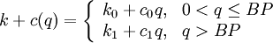
Consider the first case: Suppose the purchase price changes at the breakpoint $\,BP$

The variable cost is $\,c_{0}$ for any amount up to $\,BP$ . For an order larger than $\,BP$ , the additional amount over $\,BP$ incurs the rate $\,c_{1}$ where $\,c_{1} <c_{0}$ .

Thus, the total order cost is

$\,k+c\left(q\right),$

where

$\,c(q)=\left\{\begin{array}{ll} {c_{0} q,} & {0<q\le BP} \\ {c_{0} BP+c_{1} (q-BP),} & {q>BP} \end{array}\right.$

Alternatively, define $\,k_{0} =k$ (a constant) and 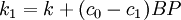$\,k_{1} =k+(c_{0} -c_{1} )BP$ (a constant!). Then, the order cost is

$\,k+c(q)=\left\{\begin{array}{ll} {k_{0} +c_{0} q,} & {0<q\le BP} \\ {k_{1} +c_{1} q,} & {q>BP} \end{array}\right.$

This function describes more elaborate economies of scale than the original fixed-plus-linear form. In a production setting, it represents costs that depend on the production quantity in a complex, nonlinear way.

The figure illustrates $\,c(q)$ for the incremental case.

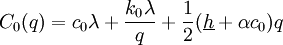
Given the revised order cost for the incremental case, the formulation proceeds as in the EOQ model. The holding cost is a bit tricky, however.

In addition to direct handling costs, which occur at rate $\,\underline{h}$ , there is also a financing cost, which occurs at rate $\,\alpha \frac{c(q)}{q}$ .

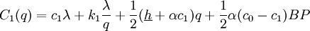
Here, $\,\alpha$ is the interest rate, and $\,\frac{c(q)}{q}$ is the average variable purchase cost. Thus, the total average cost is

$\,C(q)=\left[k+c(q)\right]\cdot \frac{\lambda }{q} +q\cdot \frac{1}{2} \cdot \left[\underline{h}+\alpha \cdot \frac{c(q)}{q} \right]$

( $\,C$ is not differentiable at $\,q=BP$ , so we cannot hope simply to differentiate to obtain the optimal solution. Also, $\,C$ is not convex.)

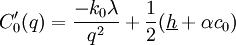
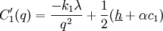
Observe that

$\,c(q)=\min \{ k_{0} +c_{0} q,k_{1} +c_{1} q\} -k,\, \, \, q>0.$

That is, $\,c(q)$ is the smaller of two positive, linear functions that cross at $\,BP$ . Therefore,

$\,C(q)=\min \{ C_{0} (q),C_{1} (q)\}$

where

$\,C_{0} (q)=c_{0} \lambda +\frac{k_{0} \lambda }{q} +\frac{1}{2} (\underline{h}+\alpha c_{0} )q$

$\,C_{1} (q)=c_{1} \lambda +k_{1} \frac{\lambda }{q} +\frac{1}{2} (\underline{h}+\alpha c_{1} )q+\frac{1}{2} \alpha (c_{0} -c_{1} )BP$

Both $\,C_{0}$ and $\,C_{1}$ have the form of the EOQ model's cost function. Both are strictly convex and differentiable, and their graphs cross at $\,BP$ . Let $\,q_{0}^{*}$ and $\,q_{1}^{*}$ be the respective minimizing values of $\,q$ . Also,

$\,C'_{0} (q)=\frac{-k_{0} \lambda }{q^{2} } +\frac{1}{2} (\underline{h}+\alpha c_{0} )$

$\,C'_{1} (q)=\frac{-k_{1} \lambda }{q^{2} } +\frac{1}{2} (\underline{h}+\alpha c_{1} )$

Evidently, 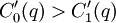$\,C'_{0} (q)>C'_{1} (q)$ , so $\,q_{0}^{*} <q_{1}^{*}$ . There remain three possible cases:

$\,q_{0}^{*} <q_{1}^{*} \le BP$
$\,q_{0}^{*} <BP\le q_{1}^{*}$
$\,BP\le q_{0}^{*} <q_{1}^{*}$

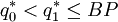
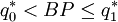
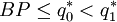
In case 1, for $\,q\ge BP$ ,

$\,C(q)=C_{1} (q)\ge C_{1} (BP)=C_{0} (BP)>C_{0} (q_{0}^{*} )$

so $\,q_{0}^{*}$ is optimal. In case 3, by a parallel argument, $\,q_{1}^{*}$ is optimal. Only in case 2 is there any doubt. In that case, calculate both $\,C_{0} (q_{0}^{*} )$ and $\,C_{1} (q_{1}^{*} )$ to determine which one is smaller.

In sum, it is easy to determine an optimal policy: Compute both $\,q_{0}^{*}$ and $\,q_{1}^{*}$ using EOQ-like formulas, compare them with $\,BP$ to determine which case applies, and if necessary (in case 2) compare their costs.

References

↑ Zipkin P. (2000) Foundations of inventory management; The McGraw-Hill Companies, Inc.

[0] Zipkin P. (2000) Foundations of inventory management; The McGraw-Hill Companies, Inc.

[1]

Revision as of 19:01, 20 May 2012 (view source) Zyatchin (Talk \| contribs) ← Older edit		Latest revision as of 23:15, 9 July 2012 (view source) Zyatchin (Talk \| contribs)
(One intermediate revision not shown)
Line 1:		Line 1:
		+	'''Russian: [http://ru.scm.gsom.spbu.ru/index.php/Экономичный_размер_заказа_с_учетом_скидки_за_прирост Экономичный размер заказа с учетом скидки за прирост]'''
		+
	In the [[Basic economic order quantity]] (EOQ) model the variable cost <math>\,c</math> is constant for orders of all sizes. However, it is common for suppliers to offer price breaks for large orders. This section shows how to extend the EOQ model to incorporate such quantity discounts. Actually, there are two kinds of discounts, incremental and all-units<ref> Zipkin P. (2000) Foundations of inventory management; The McGraw-Hill Companies, Inc.</ref>.		In the [[Basic economic order quantity]] (EOQ) model the variable cost <math>\,c</math> is constant for orders of all sizes. However, it is common for suppliers to offer price breaks for large orders. This section shows how to extend the EOQ model to incorporate such quantity discounts. Actually, there are two kinds of discounts, incremental and all-units<ref> Zipkin P. (2000) Foundations of inventory management; The McGraw-Hill Companies, Inc.</ref>.

Incremental Discounts

From Supply Chain Management Encyclopedia

Latest revision as of 23:15, 9 July 2012

References

Views

Personal tools

Navigation

Search

Toolbox

Print/export

Our Partners