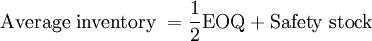
Centralized inventory planning

From Supply Chain Management Encyclopedia

Revision as of 09:44, 27 May 2011 by Germain (Talk | contribs)

(diff) ← Older revision | Latest revision (diff) | Newer revision → (diff)

Echelon inventory systems consider the case where a facility (e.g., a warehouse) serves multiple demand points (e.g., retail outlets). The basic economic order quantity model, the EOQ with trade promotion model and inventory model with uncertainty in demand and lead time are all applicable to situations where a single facility manages its own inventory without concern over inventory further downstream in the supply chain. Suppose we have a system where a single warehouse feeds two retail outlets. If the warehouse and the two retail outlets independently utilize the basic EOQ model or the inventory model with uncertainty in demand and lead time, then:

Each member of the system optimizes its own performance;
However, the overall system will suffer as no single entity is optimizing system performance.

Planners ultimately choose between one of two strategic options in designing the management of supply chain inventory:

Decentralization: This refers to a strategy where each level in the supply chain (e.g., manufacturer, wholesaler, retailer) optimizes its performance and inventory independent of other levels in the supply chain;
Centralization: This refers to a strategy where a single planner has access to information at multiple points in the supply chain and is therefore able to generate a system-wide inventory plan. In a typical retail setting, the retailer provides information about actual demand to the system-wide planner, who is then able to craft a unified channel-wide inventory policy.

A range of echelon models are available, however, many of them are complex from a mathematical perspective. Our purpose in providing a simplified model is to illustrate how an echelon model works and the potential benefits relative to single facility models. The ecehelon model we present provides a concrete example of the workings of a centralized inventory planning system.

Example: The Decentralized Model

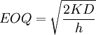
First, we shall provide and example of how a Decentralized inventory system would work. Suppose that a retailer operates one warehouse and feeds two retail stores. The unit of analysis is a case (or a carton) of a product with a value (v) of 12. Electronic ordering is used, so the fixed order cost (K) is low (2). The annual inventory carrying cost rate (c) equals 0.20. All figures will be given in terms of days. The value of h, the carrying cost of one unit (or case) per relevant time period, is therefore:

= c × v / 365
= 0.20 × 12 / 365 = 0.0066

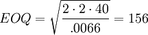
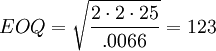
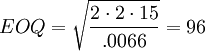
The next step in evaluating the Decentralized policy is to estimate the separate EOQs for each facility. Table 1 shows the fixed order cost and value of h (common across the three facilities), the demand per day in cases, and the EOQ values.

Table 1: Basic EOQ Inputs and Evaluations
K=2; h=.0027	Warehouse	Retail Outlet 1	Retail Outlet 2
Demand	40 cases / day	25 cases / day	15 cases / day
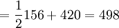
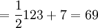
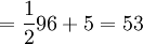
$EOQ =\sqrt{\frac{2KD}{h} }$	$EOQ =\sqrt{\frac{2\cdot 2\cdot 40}{.0066}} = 156$	$EOQ =\sqrt{\frac{2\cdot 2\cdot 25}{.0066}} = 123$	$EOQ =\sqrt{\frac{2\cdot 2\cdot 15}{.0066}} = 96$

Table 2 provides the expected lead time for each of the facilities and their respective standard decviations. For the sake of model simplicity, we assume that the standard deviation in lead time from the warehouse to each retail store is zero. Assuming otherwise increases model complexity, but does not to influence key point of illustrating the effectiveness of the Centralized policy relative to the Decentralized policy. We assume an inventory service level of 99% and therefore use a z equal to 2.33. A critical feature of this model is that the standard deviation in daily demand at the warehouse level is 61 cases per day, while that at the retail level are 3 and 2 respectively for stores 1 and 2. In a Decentralized system, each level is cleaved or cut off from other levels in terms of the information that is available to them. In this case the warehouse does not see actual demand at the retail level on a daily basis. Rather they see demand as orders from the retail stores. Daily demand at the warehouse level from retail store 1 would look like a stream that resembles 0, 0, 0, 123 (or an order equalling its EOQ), 0, 0, 0, and so on. From retail store 2, the pattern is similar, except that the order quantity will hover around its EOQ of 96. This is known as the order batching effect -- that is, when a level in a supply chain understands demand from orders placed by the next downstream level and not as actual, realized demand. The greater the number of retail outlets seviced by the warehouse, the lower the standard deviation in demand at the warehouse as orders from different stores have the ability to offset one another. Our example is thus designed to exagerate the order batching effect and thus the potential benefits of a Centralized inventory system. The sum of average inventory across retail outlets equals 620 cases.

Table 2: Safety Stock and Average Inventory Evaluation for Decentralized Inventory Planning System
	Warehouse	Retail Outlet 1	Retail Outlet 2
Lead time (LT)	Vendor to warehouse = 7 days	Warehouse to retail outlet = 1 day	Warehouse to retail outlet = 1 day
Standard deviation in lead time (σLT)	2 days	0 days	0 days
Demand	40 cases / day	25 cases / day	15 cases / day
Standard deviation in demand (σD)	61	3	2
$\mbox {Safety stock}=z\sqrt {LT \cdot \sigma D^2+D^2 \cdot \sigma LT^2}$	$2.33\sqrt {7 \cdot 61^2+40^2 \cdot 2^2}=420$	$2.33\sqrt {1 \cdot 3^2+15^2 \cdot 0^2}=7$	$2.33\sqrt {1 \cdot 2^2+15^2 \cdot 0^2}=5$
$\mbox {Average inventory } = \frac {1}{2} \,\!\mbox {EOQ} + \mbox {Safety stock}$	$= \frac {1}{2} 156 + 420=498$	$= \frac {1}{2} 123 + 7=69$	$= \frac {1}{2} 96 + 5=53$
Total system-wide average inventory = 498+69+53 = 620

Example (continued): The Centralized Model

The Centralized inventory planning system is characterized by the presence of a single entity that has access to system-wide information about inventory levels and demand. In this example, the centralized planner would have access to relevant information at both the warehouse and retail levels. In the Decentralized model, the warehouse sees demand as order batches. Under the centralized system, the vision of demand is actual demand at the retail level -- order batches are thus eliminated as a signal of demand and is replaced with information on actual demand. The simplified model for saefty stock (Table 3) utlizes the echelon lead time of 8 days. This represents the lead time from the vendor to the retail outlets. The standard deviation in lead time remains unchanged from the Decentralized model at 2 days. The assumption of zero variance in the lead time from the warehouse to the retail stores was undertaken for model simplification purposes. Demand of 40 cases per day remains unchanged. The standard deviation in daily demand decreases radically from 61 to 3.61. Two issues are relevant. First, VAR(X+Y)= VAR(X)+Var(Y)+2×Covar(X,Y). We have assumed that the covariance in demand across retail outlets is null. In reality this is generally not the case and, given, such we are overestimated the effect of the Centralized model on the change in inventory. Second, and as already mentioned, the greater the number of retail outlets served, the rgreater the ability of demand from one outlet to offset demand from another retail outlet. We are thus in a second fashion overestimating the reality of what a Centralized model can accomplish in terms of inventory reduction reality by modeling just two retail outlets. Given these cautions, safety stock is avaluated at 81 cases, the EOQ unchanged from the Decentralized model at 156, and total system inventory at 159. It is important to note that the system-wide inventory now refers to all inventory at the retail outlets, are the warehouse, and at in transit from the warehouse to the retail outlets. The system-wide inventory fell dramtically from the Decentralized model (620) to the Centralized model (159). In practice, these sort of decrease cannot be expected.

Table 3: Evaluating Average Inventory for Centralized Inventory Planning System
	Echelon (Warehouse to Retail Outlets)
Lead time (LT)	Vendor to retail outlets = 8 days
Standard deviation in lead time (σLT)	2 days
Demand	40 cases / day
Standard deviation in demand (σD)	$\sigma LT = \sqrt {3^2 + 2^2} = 3.61$
$\mbox {Safety stock} = z \sqrt {LT^e \cdot \sigma D^2+D^2 \cdot \sigma LT^{e2}}$	$2.33 \sqrt {8 \cdot 3.61^2+40^2 \cdot 2^2}=81$
$EOQ =\sqrt{\frac{2KD}{h} }$	$EOQ =\sqrt{\frac{2\cdot 2\cdot 40}{.0066}} = 156$
$\mbox {Average inventory } = \frac {1}{2} \,\!\mbox {EOQ} + \mbox {Safety stock}$	$= \frac {1}{2} 156 + 81=159$
Total average system-wide inventory = 159

Several other issues require attention:

In the analysis, all that changed was the elimination of the order batching effect. In practice, such an elimination requires additional information technology expenditures. For example, point-of-sale data needs to be used for much more tha price-look-up. It needs to be provided to the centralized inventory planning unit.
Improved efficiency in the warehousing system is generally accompanied by a shift from a Decentralized to a Centralized model. Under the former, the warehouse is used to store product that is shipped when retail store orders are obtained. Ideally, under the latter, inventory is allocated to a particular retail outlet before it arrives at the warehouse. The warehouse thus shifts from a role primarily consisting of storage to flow-through. Technically advanced retailers utilize comlpex cross docking warehouse technologies.
These systems are generally best suited to standard products with repetitive order cycles. Data is easily acquired on demand per day (or week) at different locations and may be used in evaluating demand and lead time distributions. Moving averages are commonly used to evaluate such distributions. In contrast, highly seasonal products with a single order cycle (e.g., household decorations for religious holidays) are not well suited to such systems. In many instances, retailers work with an in-store date and use warehouses as buffer locations to ensure product availability.
The question arises as to what firm in the channel should act the part of Centralized planner. That depends on the complexity of the production versus retailing and the relative meaninfulness of point-of-sale data. When the products are standard and repetitively sold, and when the retailer is large, then the manufacturer is often the Centralized planner. That is because it is more effiecient from a knowledge perspective for the manufacturer to plan its own production and to feed the retail system using final demand signals than it is for the retailer to plan production for the manufacturer. Centralized inventory planning is often associated with vendor managed inventory, however, this only holds when it is the manufacturer that is the Centralized planner. When point-of-sale-data captures less meaningful information, as in the case of rapidly changing fashion products, then it is often the retailer that is the Centralized planner. For example, the GAP and H&M fashion retail chains outsource much of their production, however, they retain control over production scheduling and the timining and flows of materials from factories to retail outlets.

Centralized inventory planning

From Supply Chain Management Encyclopedia

Example: The Decentralized Model

Example (continued): The Centralized Model

Views

Personal tools

Navigation

Search

Toolbox

Print/export

Our Partners