Basic economic order quantity
From Supply Chain Management Encyclopedia
Russian: Экономичный размер заказа
Let us consider the case of static demand.
The basic assumptions of the model
- Number of units consumed per period is a constant (demand rate);
- Price of the resource is constant;
- Carrying cost of the resource is constant;
- Order cost is constant;
- Lead time is zero.
The basic notations
 – demand rate;
 – marginal carrying costs;
 – fixed order costs;
 – order cycle time;
 – total costs per period;
 – order quantity;
 – economic order quantity.
Inventory optimal control
According to the assumptions dynamics of inventory takes the following form (Fig. 1):

Fig. 1. The dynamics of inventory in the economic order quantity model.
Since the intensity of demand for the resource is constant, the average inventory level is  units. Therefore, the total cost per unit time can be explained as a function of order volume in the form of the cost of ordering a unit of time and storage costs of the resource per unit time:
(1) 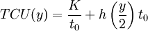 .
.
Given the dependence of the order cycle time, the intensity of demand for the resource,  , equation (1) becomes:
(2) 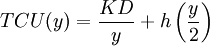 .
The first order condition for the function (2) becomes:
.
The first order condition for the function (2) becomes:
(3) 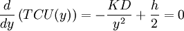 .
The second order condition for the function (2) is:
.
The second order condition for the function (2) is:
(4) 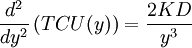 .
.
Therefore, the function is convex with respect to , where  . Then, the solution of equation (3) of the form
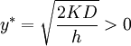
is the minimum point of . Value is the economic order quantity.
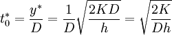
The optimal duration of order cycle becomes:
(5) 
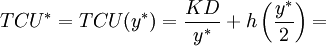
Total minimum costs per period,  , takes the following form:
(6) 
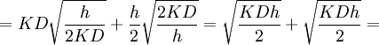
 .
.
Optimal inventory control in the economic order quantity is the following:
How much to order?. Order 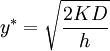 units of the resource.
When to order? After each  units of time.
Example.
On an assembly line of computers daily are consumed 50 processors. The cost of placing an order for the purchase of processors regardless of how much the party is $ 25. Carrying cost of a single processor per day is $ 0.25. What is the optimal inventory control strategy.
Solution.
 processors per day,
 for carrying one processor,
 for order.
Then economic order quantity is
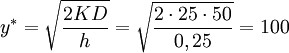
processors, and the optimal order cycle time is
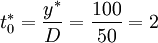 days.
days.